Remember Austin Mack's first drive against TCU?
He caught two passes for 66 yards in the first three plays, including a 50-yard bomb to get the Bucks to the one-yard line. On third and one, he dropped a slant in the back of the end zone. And then dropped almost everything else for the rest of the game.
Watching Ohio State in the red zone was frustrating all year but these three points especially hurt – the offense had the ball on the one-yard line in a big game and just could not punch it in. It seemed impossible for the Bucks to not score seven points.
Nowadays, there is a way to find out just what the Bucks missed out on that drive.
Thanks to some old statistics and new access to play-by-play data, a metric called expected points added has come to the forefront of football analytics to help solve these problems.
Expected points added (EPA) is an advanced football metric that was initially introduced in the 1970s by Virgil Carter, a former NFL quarterback and BYU graduate. It has since been reimagined by ESPN's Brian Burke and is used extensively by 538, ESPN, and Pro Football Focus.
EPA is calculated with data from previous years, where the down, distance, and field position are all taken into account to predict how many points will be scored on that offensive drive. The expected points of the drive are calculated both before and after a play, with the difference between the two being the expected points that that individual play added.
Expected points added can be an extremely useful statistic because it is based on a simple concept: not all yards are created equal. Gaining ten yards on your own 30-yard line is not the same as gaining ten yards in your opponent's red zone.
To gain a better understanding of the metric, let's circle back to our example with Mack. Before Dwayne Haskins completed that 50-yard pass, Ohio State's expected points for that drive was 2.38. After Mack came down with the pass at the one-yard line, Ohio State's expected points for the drive was 4.99, giving the play an EPA of 2.61.
After a stuffed run and two incomplete passes, however, it was fourth-and-one on the TCU one-yard line. At this point, Ohio State's expected points for the drive was 3.35, meaning the previous three plays averaged -0.55 EPA.
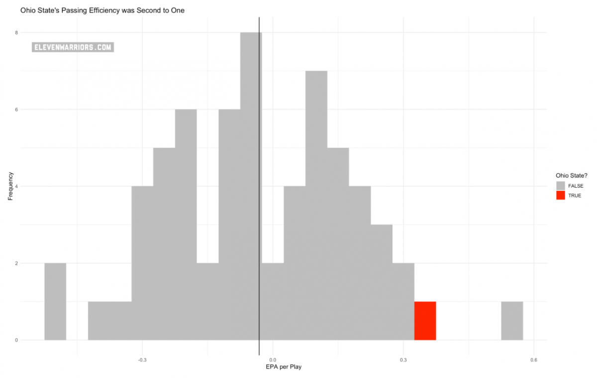
For further context, let's take a look at the EPA of nearly every play from the 2018-2019 season, with the vertical line representing the mean expected points added.

It is important to note that EPA can:
- Be negative: if you lose yards on a play, you will likely lose expected points.
- Be greater than seven: if you start a play with negative expected points and finish it in the end zone, you have contributed greater than seven expected points.
- Be less than negative seven: this one always hurts. Red zone pick sixes hurt (looking at you, Peyton Ramsey).
Expected points added goes beyond a simple calculation to show the effectiveness of a play. It can show how good (or bad) an offense or defense is, help in decision-making (such as going for it on fourth down), and even be used to track the impact individual players have on the game.
For example, Ohio State's offense was one of the best in the nation last season, but it heavily relied on Haskins. The Buckeyes had an EPA of 0.385 on passing plays, second in the Power Five to only Oklahoma's ridiculous 0.565.

Though Ohio State thrived through the air, the Bucks struggled mightily on the ground. The ground game was horrendous, giving the Buckeyes an EPA of -0.154 on running plays. The backfield struggles in Columbus handed the scarlet-and-gray just a slightly above average EPA per play despite their aerial dominance.
These numbers make sense; anyone who watched Ohio State for 20 minutes last season could have come to these conclusions. A player's individual impact, however, is a little more difficult.
For the most part, standard statistics such as yards, interceptions, touchdowns, tackles, and more are used to summarize a player's ability. These measures, however, are inherently flawed. With traditional statistics, a player that converted on fourth-down with a ten-yard catch would be given the same amount of "game effect" (yards) as a player that gained ten yards on third and long.
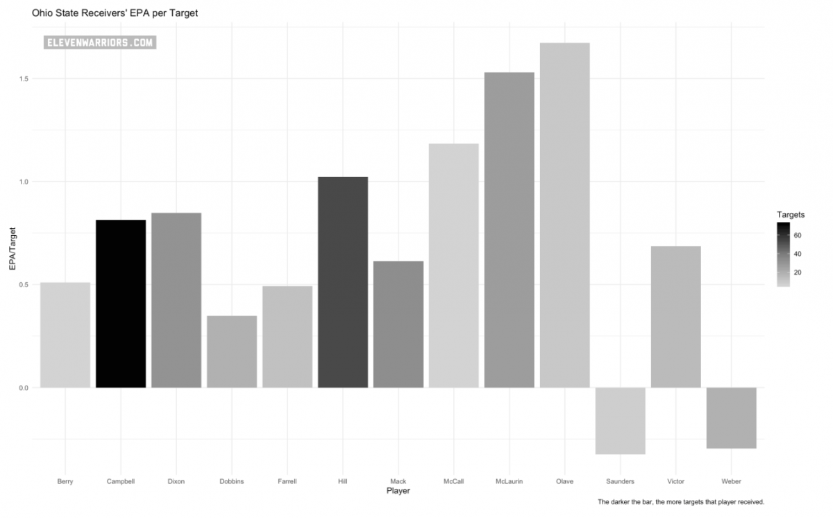
With EPA, these differences can be better measured. Ohio State's receiving corps from last season provides an interesting case. Parris Campbell and K.J. Hill both had record-breaking seasons and filled up the stat sheet. So, which of those two occupied the top spot on Ohio State's receiving corps?
Well, neither.

Instead, Terry McLaurin proved to be the most efficient, high-volume target for the Buckeyes last year. McLaurin's team-leading EPA (excluding Olave's small, albeit extremely impressive, sample size) likely assisted in his meteoric rise up draft boards.
Campbell and Hill, who combined for 160 catches last season, were constants in the offense but did not have the per-target effect that McLaurin did, which could be partially explained by their high usage rate.
While it's unlikely that Ohio State will be as effective through the air without Haskins, it is comforting to see the supporting cast he has coming back. The six top returning receivers averaged over 0.5 EPA per target, giving Justin Fields an accomplished and experienced group that will undoubtedly help him grow into the role as the face of Columbus.
Ohio State's fantastic offensive season could be explained without the use of advanced metrics, but individual performers may not be fully appreciated and comparisons between teams may lack contextual substance
The Buckeyes' receiving room is a perfect example of the fallacy of standard statistics and why EPA and other advanced metrics will continue to make their way into college football.


